Transcribed by Julien Edward Clancy (edited by Asad Lodhia, Elchanan Mossel and Matthew Brennan)

Last lecture we saw the most basic theorem about neural network approximation: that for most activation functions, including any \( \sigma \colon \mathbb{R} \to \mathbb{R} \) such that \( \sigma(x) \to 0 \) as \( x \to -\infty \) and \( \sigma(x) \to 1 \) as \( x \to \infty \), and also including the ReLU function, we can represent almost any function given enough neurons, with small error in any reasonable norm. One of the proofs relied on Fourier analysis. The simpler one was to observe that by scaling and translating to \( \sigma(\lambda x + b) \) for large \( \lambda \) and some \( b \) we can approximate the function
\[
f(x) = \chi_{[a, \infty)}(x)
\]
for every \( a \). By subtracting one of these from another we can approximate the indicator of any interval, and by standard arguments we can: 1) approximate any continuous function in the uniform sense, and 2) approximate any \( L^2 \) function in the \( L^2 \) sense. The last observation can also be adapted to Sobolev spaces, or even more detailed function classes.

An argument can be made that the result above has little to do with the practice of neural networks. Deep networks have gained currency because of their expressive power relative to their size and number of parameters — though the networks used in practice have millions of nodes, they dramatically outpace shallow networks of the same size. The first order of business of this lecture is to take a step towards explaining this.

Telgarsky’s Depth Separation: 0-1 Loss

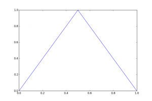
For the result we’re about to state (from a paper of Telgarsky that can be found here ) let’s consider ReLU networks. Let \( m(x) \) be the piecewise linear function that is \( 2x \) if \( x \in [0, 0.5] \), \( 2-2x \) if \( x \in [0.5, 1] \), and \( 0 \) otherwise. This looks like:

This can be computed exactly by a two- or three-layer network, depending on your notational preferences, by the expression
\[
\sigma( 2 \sigma(x) – 4 \sigma(x – 0.5) )
\]
which is a diamond-shaped network:

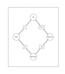
or in terms of the activation function:

where the function \( m \) is slightly offset for clarity. Since we’re looking at deep networks, what do iterates of this function look like? Here are the first four:

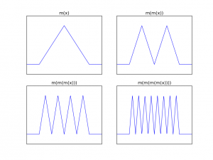
Each iteration replaces the triangle with two triangles that are half as wide (but of the same height), so \( m^{(n)}(x) \) has \( 2^n \) “teeth”. Moreover, by chaining these networks, we can obviously represent this function with \( 3n+1 \) nodes in a deep network. However, it should take very many nodes to do this in a shallow network. Intuitively, depth increases the number of oscillations multiplicatively (which is why we have an exponential number of teeth) whereas width can only do so additively. The precise (and fairly strong) version of this intuition states:

Given a function \( f \) and data points \( (x_i, y_i) \), define its classification error by
\[
R(f) = \frac{1}{n} \sum_i \chi\{\tilde{f}(x_i) \neq y_i\}
\]
where \( \tilde{f}(x) = \mathbf{1}\{ f(x_i) > 1/2 \} \) is the “sign-rounding” of \( f \). Let \( x_i = i/2^n \) and \( y_i = m^{(n)}(x_i)\) where \(y = (0,1,0,1,\ldots) \). Notice that \( R(m^{(n)}) = 0 \). If a network \( g \) has \( \ell \) layers and width \( w < 2^{(n-k)/\ell-1} \), then \( R(g) > \frac{1}{2} – \frac{1}{3 \cdot 2^{k-1}} \).

The right way to quantify the oscillatory quality of \( m^{(n)} \), for the purposes of this proof, is by how many affine pieces it has. We say a function \( f \) is \( t \)-sawtooth if it is piecewise affine with \( t \) pieces. Clearly \( m \) is \( 4 \)-sawtooth, and \( \sigma \) is \( 2 \)-sawtooth. Let’s first show a quick lemma:

If \(f\) is \(a\)-sawtooth and \(g\) is \(b\)-sawtooth, then \(f + g\) is at most \(a + b\)-sawtooth and \(f \circ g\) is at most \(ab\)-sawtooth.

[of the Lemma] Addition is simple: the “joints” of \(f\) must fall within intervals on which \(g\) is affine, and adding an affine function does not change sawtooth degree. For composition, each interval on which \(f\) is affine has as its domain at most the range of \(g\), and therefore on this interval \(f(g)\) looks like (a subset of) \(ag + b\), which is \(b\)-sawtooth. Since there are \(a\) such intervals by assumption, \(f \circ g\) is \(ab\)-sawtooth.

From this result it is clear that a depth-\(\ell\) and width-\(w\) ReLU network must produce an output that is at most \((2w)^\ell\)-sawtooth. If \(w < 2^{(n-k)/\ell-1}\) then the network computes a \(r \leq 2^{n-k}\)-sawtooth function, whereas \(m^{(n)}\) is precisely \(2^n\)-sawtooth. Now, let's examine each interval on which \(g\) is affine. If the interval contains \(p\) data points, then since \(g\) is affine on this interval it can have the correct sign for at most \(\frac{p+3}{2}\) of them. There are \(2^n\) data points overall, and if we partition them into the \(2^{n-k}\) intervals where \(g\) is constant, then \(g\) can have the correct sign for at most \(2^{n-1} + 3 \cdot 2^{n-k+1}\) of them. This means that \(R(g) > \frac{1}{2} – \frac{1}{3 \cdot 2^{k-1}} \)

It is an instructive exercise to the reader to reproduce the example for the three-class, three-output extension (where the assigned class is taken to be the maximum of the three output values).

Depth Separation: Squared Loss

More generally we are interested to approximate a function \(f \colon [0,1]^d \to \mathbb{R}\) by a ReLU network \(\tilde{f}\) of depth \(\ell\) and width \(w\), where the output level is linear and we used the squared loss to evaluate network performance. The general theme is to find structural properties of \(f\) that make it hard to approximate by shallow networks — the theorem above was the first such result we’ll see, for a certain notion of oscillatory behavior for function in one dimension. Since deep nets are most used for high dimensional problems, it is interesting to try and classify how well do networks approximated such functions.

Quadratic Functions

Recalling that shallow nets cannot have too many saw-teeth, we first obtain a more general result for quadratic functions:

Let \(p(x) = p_2 x^2 + p_1 x + p_0\). If \(g\) is \(n\)-sawtooth then there is some constant \(C > 0\) such that
\[
\lVert p – g \rVert_2^2 \geq C p_2^2 / n^4
\]

The decay looks bad, but in the end it is practically optimal. This should not discourage the reader, however, because what is important for our purposes is the relative rate of deep vs. shallow networks — this result says that shallow networks can get at best an \(n^4\) approximation rate, while deep networks can get about \(2^{4n}\).

Since \(g\) is piecewise affine let’s look at the \(L^2\) error on each of its pieces separately. On each interval \([b, b+2a]\) the error looks like
\[
\int_b^{b+2a} \left| p_2 x^2 + p_1 x + p_0 – cx – d \right|^2 \, dx
\]
where \(g_{[b,b+2a]} = cx+d\). The trick is to alter the function \(g\) on each piece individually and look at the minimum error over all affine functions; adding these over all intervals will give the lower bound we want. The minimum of the above expression is
\[
\min_{c,d} \int_b^{b+2a} \left| p_2 x^2 – cx – d \right|^2 \, dx = \min_{c,d} \int_{-a}^{a} \left| p_2 x^2 – cx – d \right|^2 \, dx
\]
since translating does not change the top coefficient of a quadratic polynomial (and everything else has been absorbed into the minimum). Scaling the integration variable by \(a\) we get
\[
\min_{c,d} a\int_{-1}^{1} \left| p_2 a^2x^2 – cax – d \right|^2 \, dx
\]
and taking out the top coefficient (again absorbing everything else) yields
\[
\min_{c,d} a^5 p_2^2 \int_{-1}^{1} \left| x^2 – cx – d \right|^2 \, dx = C a^5 p_2^2
\]
Now let \(\{[a_i,b_i]\}\) be the intervals where \(g\) is affine, and let their lengths be denoted as \(\{\ell_i\}\). Then
\[
\lVert p – g \rVert_2^2 \geq \sum C p_2^2 \ell_i^5 \geq C \frac{p_2^2}{n^4}
\]
since \(1 \leq \sum \ell_i \leq \left( \sum \ell_i^5 \right)^{1/5} \left( \sum 1 \right)^{4/5}\) so \(1/n^4 \leq \sum \ell_i^5\) by Minkowski’s inequality.

One nice interpretation of the above result is that the coefficient of the \(x^2\) term is the curvature of the function, so we’ve bounded the approximation capabilities of a neural network in terms of the curvature of the function being approximated.

Generalizing to Strongly Convex Functions

That result covers quadratic functions. Using the theory of orthogonal polynomials we can extend the result to the case of arbitrary degree polynomials, or analytic functions, or really any \( L^2 \) function. The Legendre polynomials are one such family, starting out as
\[
1, x, \frac{1}{2} \left( 3x^2 – 1 \right), \ldots
\]
This sequence can be generated in many different ways, but one simple way is to do Gram-Schmidt on the set \(\{1, x, x^2, x^3, \ldots\}\) (with the \(L^2([-1,1])\) inner product, with which we will be working for the foreseeable future).

The theory of orthogonal polynomials is a rich one but for the theorem above it suffices to work with the Legendre polynomials. Another common family is the Hermite polynomials, defined among other ways as (the normalizations of)
\[
H_n(x) = (-1)^n e^{x^2} \frac{d^n}{dx^n} e^{-x^2}
\]
or
\[
H_{n+1}(x) = 2x H_n(x) – H_n'(x)
\]
starting at \(H_0 = 1\), or implicitly by
\[
e^{2xt – t^2} = \sum_{n=0}^\infty H_n(x) \frac{t^n}{n!}
\]
or as the function \(e^{x^2}\) multiplied by the solutions to the eigenvalue problem
\[
\mathcal{F} f = \lambda f
\]
where \(\mathcal{F}\) is the Fourier transform, or many more definitions. The Legendre polynomials satisfy similarly many interesting relations. The interested reader is encouraged to learn more about these families and their applications.

Back to the topic at hand. Since the Legendre polynomials \(h_i\) are an orthonormal family, and \(\{h_0, \ldots, h_n\}\) spans exactly the space of polynomials of degree at most \(n\), the minimum from before becomes the length of an orthogonal projection onto the space of polynomials orthogonal to linear polynomials, and kills exactly the terms in an expansion corresponding to \(h_1\) and \(h_0\), the constant and linear terms. More precisely, if \(f = \sum a_i h_i\), then
\[
\min_{c, d} \int_{-1}^1 \left| f – cx – d \right|^2 = \sum_{i \geq 2} |a_i|^2 \geq |a_2|^2
\]
This gives the same curvature-type result as above, in an \(L^2\) sense. However we can relate this to more canonical properties of a function as follows. We say that a function \(f\) is \(\lambda\)-strongly convex (concave) in \(I\) if \(f”(x) \geq \lambda\) (\( \leq \lambda\)) throughout \(I\). This condition easily implies that \(f'(t) \geq f'(0) + \lambda t\) for \(t \geq 0\), and \(f'(t) \leq f'(0) + \lambda t\) for \(t \leq 0\). For any \(f\) we have
\[
a_2 = \langle f, h_2 \rangle \sim \int_{-1}^1 f(t) (3t^2 – 1) \, dt = – \int_{-1}^1 (t^3 – t) f'(t) \, dt
\]
and if \(f\) is \(\lambda\)-strongly convex this is
\[
– \int_0^1 (t – t^3) f'(t) \, dt + \int_{-1}^0 (t – t^3) f'(t) \, dt
\]
The first integral is at most \(\int_0^1 (t -t^3) (f'(0) + \lambda t) \, dt\), which by some elementary manipulation is at most \(C \lambda\). The other integral is treated identically. Therefore the \(L^2\) bound gives
\[
\lVert f – g \rVert^2 \geq C \frac{\lambda^2}{n^4}
\]

What about higher dimensions? Let \(f \in \mathcal{C}^2([0,1]^d)\). If there is a unit vector \(v\) and a connected set \(U\) such that \(\langle v, H(f)(x) v \rangle \geq \lambda\) on \(U\), where by \(H_x(f)\) we mean the Hessian matrix, then projecting along \(v\) gives strong convexity, and integrating along these one-dimensional slices gives
\[
\lVert f – g \rVert \geq C \frac{\lambda^2}{n^4} \text{Vol}(U)
\]
There’s something a little unsatisfying about this condition, however, which is that in truly high dimensions we expect functions to be intrinsically more complex than in lower dimensions, and their approximation theory should scale accordingly. Neural networks excel at high-dimensional classification in practice, and this success is surely not limited to the type of one-dimensional phenomenon described above. However, let us keep in mind that while we think of the space of, say, \(1024 \times 1024\) images as a million-dimensional vector space, it really is just a space of functions operating on two dimensions: the dimensionality of a sampling of a scene, which is exactly what a camera does, is a different notion than the dimensionality of the space on which the true scene, as a function, operates. This should be contrasted with (say) the case of DNA, where the “true” space actually does have nearly a hundred thousand dimensions.

Other Depth Separation Results

The remainder of the lecture is an overview of a few results, with the ideas of proofs sketched or absent.

Circuits

One potential model for approximability of functions (which is not exactly a neural network) is a logical circuit, with function complexity measured in circuit complexity. The idea is that we have a bit string input (in \(\{0,1\}^n\)) as the “input layer”, and at each layer we can pass the bits from the previous layer through the unary NOT or binary AND or OR gates; we call such circuits Boolean. The very strong result we want to compare to is:

( Rossman, Servedio, Tan ) For any fixed \(d\), there is a function \(f \colon \{0,1\}^n \to \{0,1\}\) computed by a linear circuit of depth \(d\) and size \(O(n)\) such that any depth-\(d-1\) circuit computing a function that agrees with \(f\) on a fraction \(1/2 + \delta\) of the possible inputs, for \(\delta > 0\), has size \(O(e^{n^{\Omega (1/d)}})\).

This result follows a long line of work in theoretical computer science, in particular work by Hastad. We note, in comparison, that the separation results obtained by Telgarsky do not provide a depth separation between depth \( d \) and \( d – 1 \) like the result above.

Eldan-Shamir

As a step in this direction we will discuss a result of Eldan and Shamir showing separation between depths 2 and 3 for pretty general activation functions. More precisely, suppose \(\sigma\) satisfies
\[
|\sigma(x)| \leq C(1 + |x|^\alpha)
\]
for some \(C\) and \(\alpha\), and assume it is sufficiently expressive in the sense that for all Lipschitz \(f \colon \mathbb{R} \to \mathbb{R}\), constant outside \([-R, R]\), and \(\delta > 0\), there exist \(a, \alpha_i, \beta_i, \gamma_i\) such that
\[
\lVert f – a – \sum_i \alpha_i \sigma(\beta_i x – \gamma_i) \rVert_\infty < \delta \]

( Eldan and Shamir ) There exists universal constants \(c, C\) with the following properties. For all \(d\) there exists a probability measure \(\mathbb{P}\) on \(\mathbb{R}^d\) and a function \(g \colon \mathbb{R}^d \to [-1,1]\) supported in \(B_{C \sqrt{d}}(0)\) expressible by a \(3\)-layer network with width \(\sim d^5\), such for any \(f\) expressible by a two-layer network with width \(c e^{c d}\) we must have
\[
\mathbb{E}\left[|f – g|^2\right] \geq c
\]

Informally, there is a universal lower bound on the approximability of \(3\)-layer networks by \(2\)-layer networks.

[Sketch] In the end the function \(g\) will be radial: \(g(x) = G(\lVert x \rVert^2)\). Equivalently, its Fourier transform will be radial. In any bounded domain \(x_i^2\) is Lipschitz so we can approximate it in one network layer by the expressivity assumption, therefore we can represent \(\lVert x \rVert^2\) in one layer as well (if we wanted to output this directly we would need another layer for summation, but since we’re using as input to the next layer this summation is build into the neuron inputs). The next layer will be used to compute \(g\). In Fourier space, choose \(\mu\) to have density \(|\phi|^2\), where \(\phi(\xi) = \mathcal{F}(\chi_{B_1(0)})(\xi)\). Clearly this is radial, and
\[
\mathbb{E}_\mu |f – g|^2 = \int |f – g|^2 |\phi|^2 \, dm = \lVert \widehat{f \phi} – \widehat{g \phi} \rVert_2^2
\]
Since \(f\) (the function we’re comparing \(g\) to) is two-layered, we have
\[
f(x) = \sum_i f_i(\langle v_i, x \rangle)
\]
where here \(f_i(x) = \sigma(x – \beta_i)\), but actually there’s enough freedom in the proof to choose different activations at each neuron in each layer provided they satisfy the properties assumed with uniform constants. By examining \(\widehat{f \phi}\) as a convolution, \(\widehat{f \phi}\) is supported in
\[
T = \cup \left(\text{span} (v_i) + B_1(0) \right)
\]
The essence is to design \(g\) such that exponentially many of these “tubes” are required to cover its support. Intuitively, we want \(\widehat{g \phi}\) to have a lot of mass away from the origin. The construction uses a randomized \(\tilde{g} = \sum_i c_i \epsilon_i g\), where \(g_i\) is radial and essentially \(\chi\{\lVert x \rVert \in \Delta_i\}\), \(\Delta_i\) is basically an interval of width \(1/N\) about \(1/d\), and \(\epsilon_i\) is Rademacher. Then \(\tilde{g} \phi \sim \sum c_i \epsilon_i g\) so \(\widehat{\tilde{g} \phi} \sim \sum \epsilon_i c_i \hat{g}_i\). It’s possible to show with not too much difficulty that \(\hat{g}_i\) has mass far away from the origin, but does \(\widehat{g \phi}\) (with some nonzero probability)? What about cancellations? Let \(P\) be the projection onto the part of the spectrum near the boundary of the ball. Then it turns out
\[
\mathbb{E}_\epsilon \left\lVert P \sum c_i \epsilon_i \hat{g}_i \right\rVert^2 = \sum_i \lVert P c_i \hat{g}_i \rVert^2
\]
which gives that there is indeed mass far from zero.