Transcribed by Joshua Pfeffer (edited by Asad Lodhia, Elchanan Mossel and Matthew Brennan)

Introduction: A Non-Rigorous Review of Deep Learning

For most of today’s lecture, we present a non-rigorous review of deep learning; our treatment follows the recent book Deep Learning by Goodfellow, Bengio and Courville.

We begin with the model we study the most, the “quintessential deep learning model”: the deep forward network (Chapter 6 of GBC).

Deep forward networks

When doing statistics, we begin with a “nature”, or function \(f\); the data is given by \(\left\langle X_i, f(X_i) \right\rangle\), where \(X_i\) is typically high-dimensional and \(f(X_i)\) is in \(\{0,1\}\) or \(\mathbb{R}\). The goal is to find a function \(f^*\) that is close to \(f\) using the given data, hopefully so that you can make accurate predictions.

In deep learning, which is by-and-large a subset of parametric statistics, we have a family of functions
\[
f(X;\theta)
\]
where \(X\) is the input and \(\theta\) the parameter (which is typically high-dimensional). The goal is to find a \(\theta^*\) such that \(f(X;\theta^*)\) is close to \(f\).

In our context, \(\theta\) is the network . The network is a composition of \(d\) functions
\[
f^{(d)}( \cdot, \theta) \circ \cdots \circ f^{(1)}( \cdot, \theta),
\]
most of which will be high-dimensional. We can represent the network with the diagram

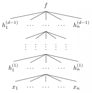
where \(h_1^{(i)},\ldots,h_n^{(i)}\) are the components of the vector-valued function \(f^{(i)}\)—also called the \(i\)-th layer of the network—and each \(h_j^{(i)}\) is a function of \((h_1^{(i-1)},\ldots,h_n^{(i-1)})\). In the diagram above, the number of components of each \(f^{(i)}\)—which we call the width of layer \(i\)—is the same, but in general, the width may vary from layer to layer. We call \(d\) the depth of the network. Importantly, the \(d\)-th layer is different from the preceding layers; in particular, its width is \(1\), i.e. , \(f = f^{(d)}\) is scalar-valued.

Now, what statisticians like the most are linear functions. But, if we were to stipulate that the functions \(f^{(i)}\) in our network should be linear, then the composed function \(f\) would be linear as well, eliminating the need for multiple layers altogether. Thus, we want the functions \(f^{(i)}\) to be non-linear.
A common design is motivated by a model from neuroscience, in which a cell receives multiple signals and its synapse either doesn’t fire or fires with a certain intensity depending on the input signals. With the inputs represented by \(x_1,\ldots,x_n \in \mathbb{R}_{+}\), the output in the model is given by
\[
f(x) = g\left( \sum a_i x_i + c \right)
\]
for some non-linear function \(g\). Motivated by this example, we define
\[
h^{(i)} = g^{\otimes}\left( {W^{(i)}}^T x + b^{(i)} \right),
\]
where \(g^{\otimes}\) denotes the coordinate-wise application of some non-linear function \(g\).

Which \(g\) to choose? Generally, people want \(g\) to be the “least non-linear” function possible—hence the common use of the RELU (Rectified Linear Units) function \(g(z) = \text{max}(0,z)\). Other choices of \(g\) (motivated by neuroscience and statistics) include the logistic function \[ g(z) = \frac{1}{1 + e^{-2\beta z}} \] and the hyperbolic tangent \[ g(z) = \tanh(z) = \frac{e^z – e^{-z}}{e^z + e^{-z}}.\] These functions have the advantage of being bounded (unlike the RELU function).

As noted earlier, the top layer has a different form from the preceding ones. First, it is usually-scalar valued. Second, it usually has some statistical interpretation: \(h_1^{(d-1)},\ldots,h_n^{(d-1)}\) are often viewed as parameters of a classical statistical model, informing our choice of \(g\) in the top layer. One example of such a choice is the linear function \(y = W^T h + b\), motivated by thinking of the output as the conditional mean of a Gaussian. Another example is \(\sigma(w^T h + b)\), where \(\sigma\) is the sigmoid function \(x \mapsto \frac{1}{1+e^x}\); this choice is motivated by thinking of the output as a probability of a Bernoulli trial with probability \(P(y)\) proportional to \(\exp(yz)\), where \(z = w^T h + b\). More generally, the soft-max is given by
\[
\text{softmax}(z)_i = \frac{\exp(z_i)}{\sum_j \exp(z_j)}
\]
where \(z = W^T h +b\). Here, the components of \(z\) may correspond to the possible values of the output, with \(\text{softmax}(z)_i\) the probability of value \(i\). (We may consider, for example, a network with input a photograph, and interpret the output \((\text{softmax}(z)_1,\text{softmax}(z)_2,\text{softmax}(z)_1)\) as the probabilities that the photograph depicts a cat, dog, or frog.)

In the next few weeks, we will address the questions: 1) How well can such functions approximate general functions? 2) What is the expressive power of depth and width?

Convolution Networks

Convolution networks , described in Chapter 9 of GBC, are networks with linear operators , namely, localized convolution operators using some underlying grid geometry. For example, consider the network whose \(k\)-th layer can be represented by the \(m \times m\) grid

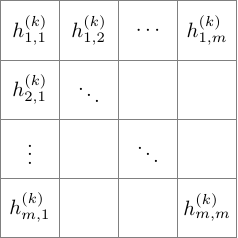
We then define the function \(h^{(k+1)}_{i,j}\) in layer \(k+1\) by convolving over a \(2 \times 2\) square in the layer below, and then applying the non-linear function \(g\):
\[
h_{i,j}^{(k+1)} = g\left( a^{(k)} h_{i,j}^{(k)} + b^{(k)} h_{i+1,j}^{(k)} + c^{(k)} h_{i,j+1}^{(k)} + d^{(k)} h_{i+1,j+1}^{(k)} \right)
\]
The parameters \(a^{(k)}, b^{(k)}, c^{(k)},\) and \(d^{(k)}\) depend only on the layer, not on the particular square \(i,j\). (This restriction is not necessary from the general definition, but is a reasonable restriction in applications such as vision.) In addition to the advantage of parameter sharing, this type of network has the useful feature of sparsity resulting from the local nature of the definition of the functions \(h\).

A common additional ingredient in convolutional networks is pooling, in which, after convolving and applying \(g\) to obtain the grid-indexed functions \(h_{i,j} ^{(k+1)}\), we replace these function with the average or maximum of the functions in a neighborhood; for example, setting
\[
\overline{h}_{i,j}^{(k+1)} = \frac{1}{4} \left( h_{i,j}^{(k+1)} + h_{i+1,j}^{(k+1)} + h_{i,j+1}^{(k+1)} + h_{i+1,j+1}^{(k+1)} \right).
\]
This technique can also be used to reduce dimension.

Models and Optimization

The next question we address is, how do we find the parameters for our networks, i.e. , which \(\theta\) do we take? Also, what criteria should we use to evaluate which \(\theta\) are better than others? For this, we usually use statistical modeling. The net \(\theta\) determines a probability distribution \(P(\theta)\); often, we will want to maximize \(P_{\theta}(y|x)\). Equivalently, we will want to minimize \[ J(\theta) = – \mathbb{E} \log P_{\theta}(y|x),\] where the expectation is taken over the data (log likelihood). For example, if we model \(y\) as a Gaussian with mean \(f(x;\theta)\) and covariance matrix the identity, then we want to minimize the mean error cost \[ J(\theta) = \mathbb{E}\left[ \left\| y – f(x;\theta) \right\|^2 \right] \] A second example to consider: \(y\) sampled according to the Bernoulli distribution with probability exponential in \(w^T h + b\), where \(h\) is the last layer; in other words, \(P(y)\) is logistic with parameter \(z = w^T h + b\).

How do you optimize \(J\) both accurately and efficiently? We will not discuss this issue in detail in this course since so far there is not much theory on this question (though such knowledge could land you a lucrative job in the tech sector). What makes this optimization hard is that 1) dimensions are high, 2) the data set is large, 3) \(J\) is non-convex, and 4) there are too many parameters (overfitting). Faced with this task, a natural approach is to do what Newton would do: gradient descent . A slightly more efficient way to do gradient descent (for us, yielding an improvement by a factor of the size of the network) is back-propagation , a method that involves clever bookkeeping of partial derivatives by dynamic programming.

Another technique that we will not discuss (but would help you find remunerative employment in Silicon Valley) is regularization . Regularization addresses the problem of overfitting, an issue summed up well by the quote, due to John Von Neumann, that “with four parameters I can fit an elephant and with five I can make him wiggle his trunk.” The characterization of five parameters as too many might be laughable today, but the problem of overfitting is as real today as ever! Convolution networks provide one solution to the problem of overfitting through parameter sharing. Regularization offers another solution: instead of optimizing \(J(\theta)\), we optimize over \[ \tilde{J}(\theta) = J(\theta) + \Omega(\theta),\] where \(\Omega\) is a “measure of complexity”. Essentially, \(\Omega\) introduces a penalty for “complicated” or “large” parameters. Some example of \(\Omega\) include the \(L_2\) or \(L_1\) (preferred to \(L_0\) for convexity reasons). In the context of deep learning, there are other ways of addressing the problem of overfitting. One is data augmentation , in which the data is used to generate more data; for example, from a given photo, more photos can be generated by rotating the photo or adding shade (A rotated dog is still a dog!). Another is noising, in which noise is added either to the data (for example, by taking a photo and blacking it out) or to the parameters.

Generative Models — Deep Boltzmann Machines

There are a number of probabilistic models that are used in deep learning. The first one we describe is an example of a graphical model . Graphical models are families of distributions that are parametrized by graphs, possibly with parameters on the edges. Since deep nets are graphs with parameters on the edges, it is natural to see whether we can express it as a graphical model. A Deep Boltzmann machine is a graphical model whose joint distribution is given by the exponential expression
\[
P(v,h^{(1)},\ldots,h^{(d)}) = \frac{1}{Z(\theta)} \exp\left( E(v,h^{(1)},\ldots,h^{(d)}) \right),
\]
where the energy \(E\) of a configuration is given by
\[
E(v,h^{(1)},\ldots,h^{(d)}) = \sum {h^{(i)}}^T W^{(i+1)} h^{(i+1)} + v^T W^{(1)} h^{(1)}.
\]
Typically, internal layers are real-valued vectors; the top and bottom layers are either discrete or real-valued.

What does this look like as a graph—what is the graphical model here? It is a particular type of bipartite graph, in which the vertices corresponding to each layer is connected only to the layer immediately above it and to the layer immediately below it.

The Markov property says that, for instance, conditional on \(h_1\), the distribution of a component of \(v\) is independent of both \(h_2,\ldots,h_d\) and the other components of \(v\). If \(v\) is discrete,
\[
P[v_i=1| h^{(1)} ] = \sigma( W_{i,*}^{(1)} h^{(1)}),
\]
and similarly for other conditioning.

Unfortunately, we don’t know how to sample from or optimize in graphical models in general, which limits their usefulness in the deep learning context.

Deep Belief Networks

Deep belief networks are computationally simpler, though a bit more annoying to define. These “hybrid” networks are essentially a directed graphical model with \(d\) layers, except the top two layers are not directed: \(P(h^{(d-1)},h^{(d)})\) is given by
\begin{equation}
P(h^{(d-1)},h^{(d)}) = Z^{-1} \exp\left( {b^{(d)}}^T h^{(d)} + {b^{(d-1)}}^T h^{(d-1)} + {h^{(d-1)}}^T W^{(d)} h^{(d)} \right)
\label{star}
\end{equation}
For the other layers,
\begin{equation}
P( h^{(k)} | h^{(k+1)}) = \sigma^{\otimes}\left(b^{(k)} + {W^{(k+1)}}^T h^{(k+1)}\right).
\label{starr}
\end{equation}
Note that we are going in the opposite direction that we were before. However, we have the following fact: if \(h^{(k)}, h^{(k+1)} \in \{0,1\}^n\) are defined by (\ref{star}), then they satisfy (\ref{starr}).

Note that we know how to sample the bottom layers conditional on layers directly from above; but for inference we also need the conditional distribution of the output given the input.

Finally, we emphasize that, while the \(k\)-th layer in the deep Boltzmann machine depends on layers \(k+1\) and \(k-1\), in deep belief, if we condition only on layer \(k+1\), we can accurately generate the \(k\)-th layer (not conditional on other layers).

Plan for the Course

In this class, the main topics we plan to discuss are

• the expressive power of depth,
• computational issues, and
• simple analyzable generative models.

The first topic addresses the descriptive power of networks: what functions can be approximated by networks? The papers we plan to discuss are

• “Approximations by superpositions of sigmoidal functions” by Cybenko (89).
• “Approximation capabilities of multilayer feedforward networks” by Hornik (91).
• “Representation Benefits of Deep Forward Networks” by Telgarsky (15).
• “Depth Separation in Relu Networks” by Safran and Shamir (16)
• “On the Expressive Power of Deep Learning: A Tensor Analysis” by Cohen, Or, Shashua (15).

The first two papers, which we will start to describe later in this lecture, prove that “you can express everything with a single layer” (If you were planning to drop this course, a good time to do so would be after we cover those two papers!). The subsequent papers, however, show that this single layer would have to be very wide, in a sense we will make precise later.

Regarding the second topic, hardness results we discuss in this course will likely include

• “On the computational efficiency of training Neural Networks” by Livni, Shalev Schwartz and Shamir (14).
• “Complexity Theory Limitation for learning DNFs” by Danieli
  and Shalev-Schwartz (16).
• “Distribution Specific Hardness of learning Neural Networks” by Shamir (16).

On the algorithmic side:

• “Guaranteed Training of Neural Networks using Tensor Methods” by Janzamin, Sedghi and Anandkumar (16).
• “Train faster, generalize better” by Hardt, Recht and Singer.

Finally, papers on generative models that we will read will include

• “Provable Bounds for Learning Some Deep Representations” by Arora et. al (2014).
• “Deep Learning and Generative Hierarchal models” by Mossel (2016).

Again, today we will begin to study the first two papers on the first topic—the papers by Cybenko and Hornik.

The Theorems of Cybenko and Hornik

In his 1989 paper, Cybenko proved the following result.

In the above theorem, \(C_n([0,1]) = C([0,1]^n)\) is the space of continuous functions from \([0,1]^n\) to \([0,1]\) with the metric \(d(f,g) = \sup|f(x)-g(x)|\).

Hornik proved the following generalization of Cybenko’s result.

In the above Theorem, the space \(L^p(\mu)\) is the space of functions \(f\) with \(\int |f|^p d\mu < \infty\) with metric \(d(f,g) = \left( \int |f-g|^p d\mu \right)^{1/p}\). To begin the proof, we need a crash course in functional analysis.

Why is this theorem useful in our context? Our proof of Cybenko and Hornik’s results is a proof by contradiction using the Hahn-Banach extension theorem. We consider the subspace \(U\) given by \(\{ \sum \alpha_j \sigma(w_j^T x + b_j)\}\), and we assume for contradiction that \(\overline{U}\) is not the entire space of functions. We conclude that there exists a continuous linear map \(L\) on our function space that restricts to \(0\) on \(\overline{U}\) but is not identically zero. In other words, to prove the desired result, it suffices to show that any continuous linear map \(L\) that is zero on \(U\) must be the zero map.

Now, classical results in Functional analysis state that a continuous linear functional \(L\) on \(L^p(\mu)\) can be expressed as
\[
L(f) = \int f g \,d\mu
\]
for some \(g \in L^q(\mu)\), where \(\frac{1}{p} + \frac{1}{q} = 1\). A continuous linear functional \(L\) on \(C(X)\) can be expressed as
\[
L(f) = \int f \,d\mu(x),
\]
where \(\mu\) is a finite signed measure supported on \(X\).
We can find similar expressions for linear functionals on the other spaces considered in the theorems of Cybenko and Hornik.

Before going into the general proof, consider the (easy) example in which our function space is \(L^p(\mu)\) and \(\sigma(x) = \mathbf{1}(x \geq 0)\). How do I show that, if \(L(f) = 0\) for all \(f\) in the set defined in the theorem, then the function \(g \in L^q(\mu)\) associated to \(L\) must be identically zero? By translation, we obtain from \(\sigma\) the indicator of any interval, i.e., we can show that \(\int_a^b g d\mu =0\) for any \(a < b\). Since \(\mu\) is finite (\(\sigma\)-finiteness is enough here), \(g\) must be zero, as desired. Using this example as inspiration, we now consider the general case in the setting of Cybenko's theorem. We want to show that \[ \int_{\mathbb{R}^k} \sigma(w^t x + b) d\mu(x) = 0 \forall w,b \] implies that \(\mu = 0\). First, we reduce to dimension \(1\) using the following Fourier analysis trick: defining the measures \(\mu_a\) as \[ \mu_a(B) = \mu(x: a^t x \in B),\] we observe that \[ \int_R \sigma(w^t x + b) d\mu_a(x) = 0 \] Moreover, if we can show that \(\mu_a \equiv 0\) for each \(a\), then \(\mu \equiv 0\) (``a measure is defined by all of its projections''), since then \[ \hat{\mu}(a) = \int_{\mathbb{R}^k} \exp(i a^t x) d\mu(x) = \int_{\mathbb{R}} \exp(it) d\mu_a(t) = 0 \Rightarrow \hat{\mu} =0 \Rightarrow \mu = 0. \] (Note that we used the finiteness of \(\mu\) here.) Having reduced to dimension \(1\), we employ another very useful trick (that also uses the finiteness of \(\mu\))---the convolution trick. By convolving \(\mu\) with a small Gaussian, we obtain a measure that has a density, letting us work with Lebesgue measure. We now sketch the remainder of the proof. By our convolution trick, we have \begin{equation} \int_{\mathbb{R}^k} \sigma(w^t x + b) h(x) dx = 0 \quad \forall w,b \label{con} \end{equation} and want to show that the density \(h = 0\). Changing variables, we rewrite the condition (\ref{con}) as \[ \int_{\mathbb{R}} \sigma(t) h(wt+b) dt = 0 \quad \forall w \neq 0,b \] To show that \(h=0\), we use the following tool from abstract Fourier analysis. Let \(I\) be the closure of the linear space spanned by all the \(h(wt+b)\). Since \(I\) is invariant under shifting our functions, it follows that it is invariant under convolution; in the language of abstract Fourier analysis, \(I\) is an ideal with respect to convolution. Let \(Z(I)\) denote the set of all \(\omega\) at which the Fourier transform of all functions on \(I\) vanish; then \(Z(I)\) is either \(\mathbb{R}\) or \(\{0\}\) since if \(g(t)\) is in the ideal then so is \(g(t w)\) for \(w \neq 0\). If \(Z(I) = \mathbb{R}\) then all the functions in the ideal are constant \(0\) as needed. Otherwise, \(Z(I) = \{0\}\), then, by Fourier analysis, \(I\) is the set of all functions with \(\hat{f}(0) = 0\); i.e, all non-constant functions. But if \(\sigma\) is orthogonal to all non-constant functions, then it follows that \(\sigma = 0\). We conclude that \(Z(I) = \mathbb{R}\), i.e. , \(h = 0\), completing the proof.